Why is Multitasking Not Magic? - Process Scheduling

Introduction

Ever wondered how your computer manages to run your music player, web browser, code editor, and chat application all at the same time? It might seem like magic, but there’s actually a lot of careful planning happening behind the scenes. Your operating system is constantly making decisions about which process gets to use the CPU next, and for how long.

Today, we’ll explore the world of process scheduling - the algorithms and strategies that make multitasking possible. We’ll see why some applications feel snappy while others seem sluggish, and understand the trade-offs operating systems make to keep everything running smoothly.

The execution timeline of a process might not be understandable at times for complex algorithms, so I highly recommend you to have the visualizer open in a separate tab while reading this post. It will help you visualize the execution of processes and understand the scheduling algorithms better. Also, keep a pen and paper handy to jot down calculations as we go along!

Table of Contents

• The Scheduling Problem
• Understanding Process States and Schedulers
• Key Performance Metrics
• Preemptive vs Non-Preemptive Scheduling
• Scheduling Algorithms
  • First Come First Serve (FCFS)
  • Shortest Job First (SJF)
  • Priority Scheduling
  • Round Robin (RR)
  • Multilevel Queue Scheduling
  • Multilevel Feedback Queue Scheduling
• Multiprocessor Scheduling
• Coming Up Next

The Scheduling Problem

Imagine you’re a manager at a busy restaurant. You have multiple orders coming in, different dishes that take varying amounts of time to prepare, and a limited number of chefs. How do you decide which order to prepare first? Do you go in the order they arrived? Focus on the quickest dishes first? Or maybe prioritize VIP customers?

This is exactly the problem your operating system faces, except instead of food orders, it’s managing processes (running programs), and instead of chefs, it has CPU cores. The goal is to keep everyone happy - users want their applications to be responsive, and the system wants to make efficient use of its resources.

Understanding Process States and Schedulers

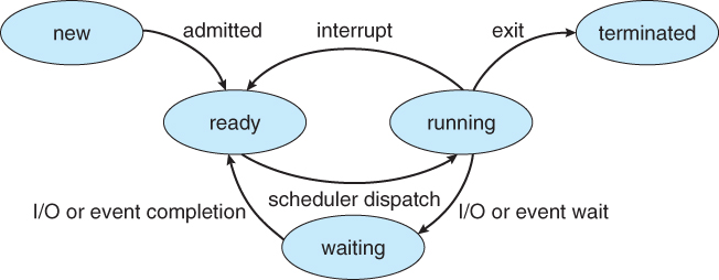
Before diving into scheduling algorithms, let’s understand how processes move through different states:

• New: Process is being created
• Ready: Process is loaded in memory and waiting for CPU time
• Running: Process is currently executing on the CPU
• Waiting: Process is blocked, waiting for some event (like I/O completion)
• Terminated: Process has finished execution

The operating system uses different types of schedulers to manage these transitions:

You can see all the process states in this diagram from the University of Illinois at Chicago.

Long-term Scheduler (Job Scheduler)

Think of this as the bouncer at a club. It decides which processes get admitted into the system and loaded into memory. It controls the degree of multiprogramming - how many processes are active at once.

Short-term Scheduler (CPU Scheduler)

This is like a traffic controller at a busy intersection. It decides which process from the ready queue gets to use the CPU next. This happens very frequently - potentially thousands of times per second.

Medium-term Scheduler

Acts like a parking valet, moving processes in and out of memory as needed to manage system resources effectively.

Key Performance Metrics

When evaluating scheduling algorithms, we use several important metrics:

• Arrival Time (AT): When the process enters the ready queue
• Burst Time (BT): How long the process needs the CPU
• Completion Time (CT): When the process finishes execution
• Turnaround Time (TAT): Total time from arrival to completion $$TAT = CT - AT$$
• Waiting Time (WT): Time spent waiting in the ready queue $$WT = TAT - BT$$
• Response Time (RT): Time from arrival until first CPU allocation
• Throughput: Number of processes completed per time unit

Our goal is to maximize CPU utilization and throughput while minimizing turnaround time, waiting time, and response time.

Preemptive vs Non-Preemptive Scheduling

Non-Preemptive Scheduling

Once a process starts running, it keeps the CPU until it voluntarily gives it up (by finishing or requesting I/O). It’s like letting someone finish their entire presentation without interruption.

Pros:

• Simple to implement
• No overhead from context switching
• Predictable behavior

Cons:

• One long process can hold up everything else
• Poor responsiveness for interactive applications

Preemptive Scheduling

The operating system can forcibly take the CPU away from a running process. It’s like having a timer that ensures everyone gets a fair chance to speak.

Pros:

• Better responsiveness
• Fairer resource sharing
• Can prioritize urgent tasks

Cons:

• More complex to implement
• Overhead from frequent context switches
• Potential for process starvation

Scheduling Algorithms

Visualize all the scheduling algorithms using the visualizer as we go along! You will get the Gantt charts as well.

Let’s explore the main scheduling algorithms with practical examples.

First Come First Serve (FCFS)

FCFS is the simplest scheduling algorithm - processes are executed in the order they arrive, just like a queue at the grocery store.

Example:

Let’s say we have three processes:

Process	Arrival Time	Burst Time
P1	0	6
P2	1	2
P3	2	8

Execution Timeline:

0----------6----8----------16
|----P1----|-P2-|----P3----|

Calculations:

• P1: $TAT = 6-0 = 6$, $WT = 6-6 = 0$
• P2: $TAT = 8-1 = 7$, $WT = 7-2 = 5$
• P3: $TAT = 16-2 = 14$, $WT = 14-8 = 6$

$$\text{Average TAT} = \frac{6+7+14}{3} = 9$$ $$\text{Average WT} = \frac{0+5+6}{3} = 3.67$$

The Convoy Effect Problem: Imagine you’re at a fast-food restaurant behind someone ordering for their entire office. Even though you just want a simple burger, you have to wait for their massive order to complete. Similarly, if a long process arrives first, all shorter processes must wait, leading to poor average waiting times.

Shortest Job First (SJF)

SJF prioritizes processes with the shortest burst time, like serving the quickest orders first at a restaurant.

Non-Preemptive SJF Example:

Using the same processes but scheduling shortest jobs first:

Process	Arrival Time	Burst Time
P2	1	2
P1	0	6
P3	2	8

Execution Timeline:

0----------6----8----------16
|----P1----|-P2-|----P3----|

Wait, this looks the same! That’s because P1 arrived first and was already running when P2 arrived. In non-preemptive SJF, we can’t interrupt P1.

Preemptive SJF (Shortest Remaining Time First):

Now we can interrupt processes when a shorter job arrives:

0--1--3------9------17
|P1|P2|--P1--|--P3--|

Calculations for Preemptive SJF:

• P1: $TAT = 9-0 = 9$, $WT = 9-6 = 3$
• P2: $TAT = 3-1 = 2$, $WT = 2-2 = 0$
• P3: $TAT = 17-2 = 15$, $WT = 15-8 = 7$

$$\text{Average TAT} = 8.67\text{, Average WT} = 3.33$$

SJF gives optimal average waiting time, but it’s hard to predict burst times in practice.

Priority Scheduling

Each process gets a priority value, and the CPU goes to the highest priority process. It’s like having VIP lanes at airports.

Example with Preemptive Priority:

Process	Arrival	Burst	Priority
P1	0	4	2
P2	1	3	1
P3	2	1	4
P4	3	5	3

(Lower priority number = higher priority)

Execution Timeline:

0--1------4--5---------9
|P1|--P2--|P3|--P1+P4--|

P2 preempts P1 when it arrives (higher priority), then P1 resumes after P2 completes.

The Starvation Problem: Low-priority processes might never get CPU time if high-priority processes keep arriving.

Solution: Aging - gradually increase the priority of waiting processes over time.

Round Robin (RR)

Round Robin gives each process a fixed time slice (quantum), then moves to the next process in a circular fashion. It’s like taking turns on a playground swing with a timer.

Example with Time Quantum = 2:

Process	Arrival	Burst
P1	0	4
P2	0	3
P3	0	1

Execution Timeline:

0--2--4--5----6--8
|P1|P2|P3|-P1-|P2|

Process Flow:

1. P1 runs for 2 units (quantum), then goes to back of queue
2. P2 runs for 2 units, then goes to back of queue
3. P3 runs for 1 unit (completes), removed from queue
4. P1 runs for remaining 2 units (completes)
5. P2 runs for remaining 1 unit (completes)

Choosing Time Quantum:

• Too small: High context switch overhead, system spends more time switching than working
• Too large: Becomes like FCFS, poor responsiveness
• Sweet spot: Usually 10-100 milliseconds

Multilevel Queue Scheduling

Processes are permanently assigned to different queues based on their characteristics. Each queue can have its own scheduling algorithm.

Example Setup:

• Queue 1 (Foreground/Interactive): Uses Round Robin with quantum = 2
• Queue 2 (Background/Batch): Uses FCFS
• Priority: Queue 1 always executes before Queue 2

Process	Queue	Arrival	Burst
P1	1	0	4
P2	1	0	3
P3	2	0	6
P4	2	0	8

Execution:

Queue 1 processes (P1, P2) execute first using Round Robin, then Queue 2 processes (P3, P4) execute using FCFS.

Multilevel Feedback Queue Scheduling

Unlike multilevel queue, processes can move between queues based on their behavior. It’s like a smart system that learns from how processes behave.

Typical Setup:

• Queue 0: Round Robin with quantum = 4
• Queue 1: Round Robin with quantum = 8
• Queue 2: FCFS

Rules:

1. New processes start in Queue 0
2. If a process uses its full time quantum, it moves to the next lower queue
3. If a process doesn’t use its full quantum (I/O bound), it stays in the same queue
4. Higher queues have priority over lower queues

This naturally separates:

• I/O-bound processes (interactive): Stay in high-priority queues
• CPU-bound processes (batch): Move to lower-priority queues

Multiprocessor Scheduling

Modern systems have multiple CPU cores, adding complexity to scheduling decisions.

Asymmetric Multiprocessing

One “master” processor handles all scheduling decisions and system activities. Other processors only execute user processes.

Pros:

• Simple to implement
• No data sharing conflicts

Cons:

• Master processor can become a bottleneck
• Doesn’t scale well with many processors

Symmetric Multiprocessing (SMP)

All processors are equal and can make scheduling decisions.

Global Queue Approach

All processors share a single ready queue.

Pros:

• Automatic load balancing
• Simple conceptually

Cons:

• Queue access requires locking (performance bottleneck)
• Poor cache locality as processes can run on different processors

Per-CPU Queue Approach

Each processor has its own ready queue.

Pros:

• No locking overhead
• Better cache locality
• Scales well

Cons:

• Load imbalancing issues
• More complex load balancing required

Load Balancing Techniques:

• Push migration: Periodically check for imbalanced queues and move processes
• Pull migration: Idle processors “steal” work from busy processors

Processor Affinity: Processes tend to run better on the same processor due to cache warmth. The scheduler tries to keep processes on the same processor when possible.

Real-World Examples

Windows: Uses a multilevel feedback queue with 32 priority levels. Interactive processes get priority boosts to improve responsiveness.

Linux: Uses the Completely Fair Scheduler (CFS), which tries to give each process an equal share of CPU time using a red-black tree data structure.

macOS: Uses a multilevel feedback queue system similar to traditional Unix, with priority adjustments for interactive processes.

Coming Up Next

Process scheduling is crucial for system performance, but what happens when processes need to share resources and end up waiting for each other indefinitely? In our next post, we’ll explore “Deadlocks: When Your OS is in a Toxic Relationship” - understanding how systems can get stuck and the strategies operating systems use to prevent, avoid, detect, and recover from these problematic situations.